Introduction

Simulation can be a great way to understand an empirical quantitative problem. In this post, let’s see how we can generate binary (dummy) outcome variables for logistic regression. A binary variable is only made of zeros and ones.

To simulate binary data, we follow three main steps

• Build a linear model
• Transform the outcome of the model into probabilities
• From the probabilities, draw binary data (from a binomial distribution)

The Model

Imagine that we want to simulate the probability of getting a job. This is our outcome variable.

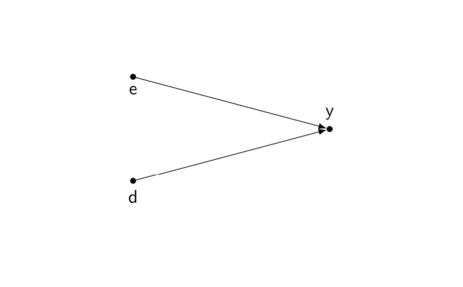
We will build the following simple model: getting a job is affected by education (\(e\)) and discrimination (\(d\)). In this model, education and discrimination are uncorrelated.

We simulate this DAG with a simple linear model

\begin{equation} \gamma_{i} = \beta_{1} e_{i} + \beta_{2} d_{i} + \epsilon_{i} \end{equation}

Let Education (\(e\)) be a standardised normal variable and Discrimination (\(d\)) a binary variable indicating if the person belongs to group \(D\). Let’s generate group membership with a binomial distribution, with 50% of chances of belonging to group \(D\).

library(tidyverse)

N=500
education = rnorm(N,0,1)
d = rbinom(N, 1, 0.5)

Let’s give the following values to \(\beta_{1}\) and \(\beta_{2}\)

\begin{equation} \gamma_{i} = ( 1.5 \cdot e_{i}) - (2 \cdot d_{i}) + \epsilon_{i} \end{equation}

Education increases the chances of getting a job, while discrimination reduces the chances of getting a job.

Let’s include an error term to the equation

error = rnorm(N) # random error term
y = 1.5*education + (-2*d) + error

We can now transform this outcome \(y\) (which we conceive being on a logit scale), into a probability, which we call \(\pi_{i}\), using the following transformation.

\begin{equation} \pi_{i} = \frac{1}{1 + \text{exp}^{-\gamma_{i}} } \end{equation}

Which is the same equation as

\begin{equation} \pi_{i} = \frac{\text{exp}^{\gamma_{i}} }{1 + \text{exp}^{\gamma_{i}} } \end{equation}

Note that this is the standard logistic model

\begin{equation} \pi_{i} = \frac{1}{1 + \text{exp}^{- \mathbf{X\beta}} } \end{equation}

The logistic transformation is not the only transformation possible to turn values into probabilities (e.g. arcsine transformation).

Generate Probabilities

The function plogis is the logistic equation shown above

y_proba = plogis(y)

We now have a probability for each row, each case / individual, that is a function of education and discrimination.

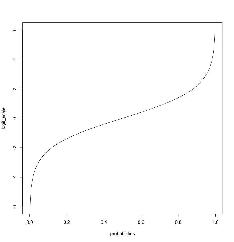
The logistic transformation transform the values we generated from our model (which we takes as being log-odds) into probabilities. Note that probabilities are bounded \([0,1]\) while our log-odds (“logit values”) goes from minus infinity to infinity, \([- \infty, \infty]\)

You can generate this plot with the following code

logit_scale = seq(-6, 6, by = 0.1)
plot(plogis(logit_values), logit_scale, xlab = 'probabilities', type = 'n')
lines(plogis(logit_values), logit_scale)

Generate Binary Outcome

Let’s now finally generate the binary outcome for the logistic regression.

We use the R function rbinom generate data based on the Binomial distribution.

y_dummy = rbinom(n = N, size = 1, prob = y_proba)

The function rbinom generates 0 and 1 based on the probabilities that we input (y_proba). For instance, a case/row/individual with a probability of 0.5 means that it has 50% of getting either 0 or 1.

We now have a dummy variable we can use to test a logistic regression model. Let’s put everything into a dataset.

df_sim = data.frame(id = 1:N, education, d, y, y_proba, y_dummy)

The dataset looks like this (you will have different values)

Logistic Regression

Finally we can run a logistic regression on the simulated dataset

glm_model1 = glm(y_dummy ~ education + d, data = df_sim, family = 'binomial')

The coefficients are expressed in log-odds, we can retrieve the odds by simply taking the exponential of the coefficients.

exp(coef(glm_model1))

We can convert the coefficient to probabilities with the predict() function

pred_prob_repsonse = predict(glm_model1, type = "response")

Check if our predicted probabilites from the model are close to the true probabilities we generated.

head( cbind(df_sim, pred_prob_repsonse) )

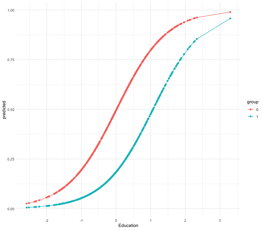
Let’s plot the predicted probabilities with the library(ggeffects).

library(ggeffects) # you need to install this library

# predicted probabilities
g_pred1 = ggpredict(glm_model1, terms = c('education[all]', 'd')) 
g_pred1 = as.data.frame(g_pred1)

# ggplot
ggplot(g_pred1, aes(x, predicted, colour = group))  +
  geom_point() + geom_line() + xlab('Education') + 
  scale_x_continuous(breaks = seq(-3,3,by=1)) + theme_minimal()

We can also compare the results to a simple OLS regression on the binary outcome (i.e. linear probability model)

lm_model1 = lm(y_dummy ~ education + d, data = df_sim)
pred_lm_model = predict(lm_model1)

What do you see?

plot(pred_lm_model, pred_prob_repsonse)

The full code

library(tidyverse)
library(ggeffects)

N=500
education = rnorm(N,0,1)
d = rbinom(N, 1, 0.5)
error = rnorm(N) # random error term

# the model
y = 1.5*education + (-2*d) + error

# logistic transformation
y_proba = plogis(y)

# draw binary data from binomial distribution
y_dummy = rbinom(n = N, size = 1, prob = y_proba)

# dataframe
df_sim = data.frame(id = 1:N, education, d, y, y_proba, y_dummy)

# the logistic regression model
glm_model1 = glm(y_dummy ~ education + d, data = df_sim, family = 'binomial')

# summary, odds and confidence intervals
summary(glm_model1)
exp(coef(glm_model1))
confint(glm_model1)

# predicted probabilities
g_pred1 = ggpredict(glm_model1, terms = c('education[all]', 'd')) 
g_pred1 = as.data.frame(g_pred1)

# ggplot
ggplot(g_pred1, aes(x, predicted, colour = group))  +
  geom_point() + geom_line() + xlab('Education') + 
  scale_x_continuous(breaks = seq(-3,3,by=1)) + theme_minimal()