Short Guide to Utility Functions (with R Examples)

In this post I will present some common Utility functions with examples using R. This post is based on the book Intermediate. Microeconomics. A Modern Approach. Eighth Edition by Hal R. Varian.

You can find the code of this post here

https://github.com/giacomovagni/gcodes/blob/master/gcode_project/2023-05-09-cobbs-douglas.R

The concept of Utility is an old concept stemming from English utilitarian philosophy (e.g. Betham, JS Mill). It denotes very generally the idea of happiness or enjoyment. When it is too hard to put an exact number on happiness (e.g. on a scale from $1$ to $10$ , how much do you like apples and oranges), then we have to resort to ranking (e.g. I prefer apples to oranges, but I do not know by how much). This is a complex problem in economics, and if you are interested in it, search for “ordinal vs cardinal Utility”.

The idea of a “Utility function” is to give Utility or Happiness¹ a functional form. The simplest form is the additive form. Imagine that we have two goods (apples and oranges), called $x_{1}$ and $x_{2}$ ; we can assume that our happiness from their consumption simply adds up, such as

U (X, Y) = x_{1} + x_{2}

If I derive one point of enjoyment from $x_{1}$ and one point from $x_{2}$ , then consuming one unit of each will get me $2$ points of Utility (also called “utils”). In this case, what we assume is that Utility sums up.

Economists have categorised different types of functional forms of Utility, for instance

(Perfect) substitute
(Perfect) complement
“Bads”
Quasi-linear
Cobbs-Douglas

And many more.

In this post, I will focus mainly on the Cobbs-Douglas function and on Perfect substitute.

One of the most challenging tasks of consumer theory is choosing a sensible Utility function. This is because the functional form must accurately reflect how individuals make economic decisions in the real world.

Many social scientists have simply given up on this, arguing it is impossible. Nevertheless, despite the difficulties, economists have tried hard to model human decisions in economic settings.

Can we really model mathematically human behavior at the micro-level? What do you think?

Perfect substitute

The form $U (X, Y) = x_{1} + x_{2}$ denotes a perfect substitute Utility form. An important idea behind this form is that what matter for our Utility, in the end, is the total number of units consumed.

For instance, imagine that I need to do $1$ hour of sport every day to have a certain level of happiness. Playing one hour of football, one hour of tennis, or $30$ minutes of both, is the same to me.

In the end, spending a certain energy level (or burning a certain number of calories) is what matters.

We can have different equivalence regarding energy burn between sports; for instance, $1$ hour of wrestling burns $900$ calories, while $1$ hour of football burns $600$ calories.

A general functional form for substitute goods looks like this

U (x_{1}, x_{2}) = a x_{1} + b x_{2}

where $a$ and $b$ are multiplicative factors representing the effects on Utility (see Varian p.61).

Therefore, $- \frac{a}{b}$ represents the substitution rate between the two goods or the two activities. If tennis and badminton have the same “values” for burning calories, let’s say 1-to-1, then my substitution rate is $- 1$ .

For a “Utility” of $60$ minutes of sport (or for burning a certain number of calories), giving up $1$ minute of tennis would need to be compensated by $1$ minute of badminton.

We have a substitution plot like this one

We can see that the substitution rate is constant. In other words, the slope $- \frac{a}{b}$ does not vary between different combinations of tennis and badminton.

My willingness to exchange tennis for badminton does not change, if I have already played 15 minutes of tennis or 45 minutes.

However, this is not always the case and functions like the Cobbs-Douglas model exactly this; the rate of substitution is allowed to differ according to different combinations. More below.

Indifference Curve & Marginal Utility

Before proceeding, let’s discuss the idea of “indifference curve”.

In the example of burning calories, we can think of the burnt calories as my Utility. For example, $1000$ calories burnt is $1000$ utils (we can imagine that each calorie burnt increases my happiness).

The indifference curve represents the combinations between $x_{1}, x_{2}$ for a fixed level of Utility.

For instance, if I want to burn $300$ calories, what are the combinations of tennis and badminton needed to maintain this level of Utility (or this level of calorie expenditure)?

For simplification, let’s say that $1$ minute of tennis or badminton burns $5$ calories, so $60$ minutes will burn $300$ calories.

I can have many combinations respecting this Utility level; $60$ minutes of tennis and $0$ minutes of badminton, or $(60, 0)$ , $(45, 15)$ , $(30, 30)$ , $(0, 60)$ . All these combinations are equivalent in terms of Utility.

The slope of this line is still $- \frac{b}{a}$ which here is $- 1$ .

The indifference curve is a curve on which I can trade off one good for another and remain at the same level of Utility or happiness.

I can have different levels of happiness of course. I would be even happier if I burned $450$ calories instead of $300$ . Generally, the greater the consumption of a good/service/activity, the greater the happiness (up to a point ).

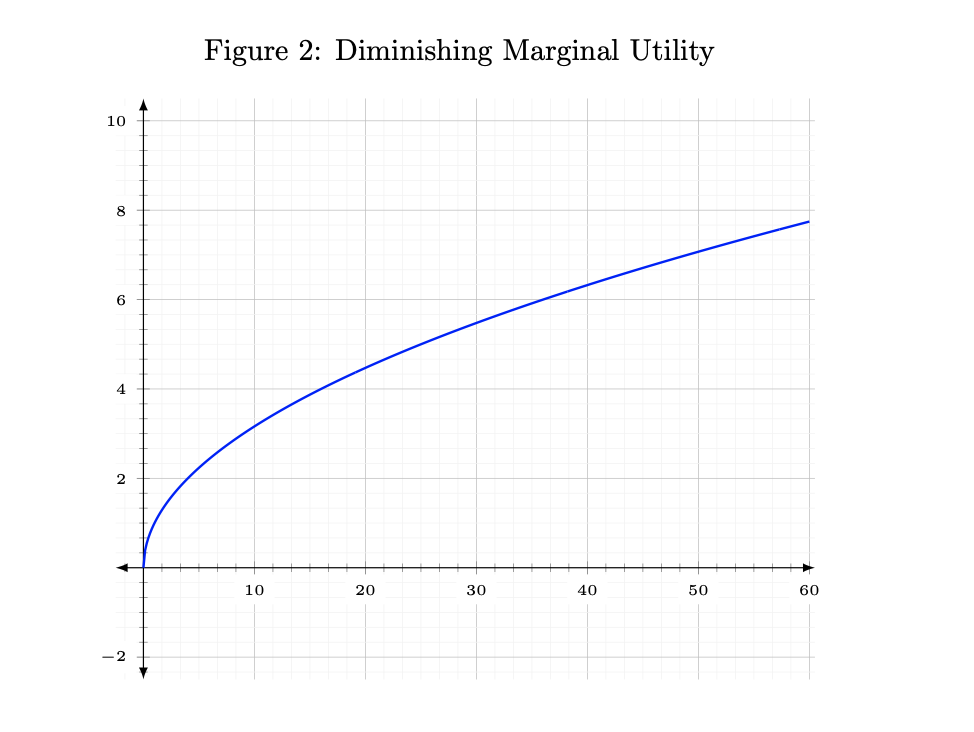
Moreover, economists recognize that the enjoyment of a good is not generally linear but follows diminishing returns. The first $10$ calories I burn provide me with much greater happiness than the calories I continue to burn after that. For each extra unit of activity, the “returns” on my Utility diminishes. My happiness is still increasing but with less and less benefits. (The first coffee provides me with more energy than the sixth one).

This is a very powerful idea. However, eating ten piece of cakes may no longer add to our happiness but instead cause discomfort. One way to approach this is to acknowledge that we rarely reach these “extreme” points and, in our daily lives, more is typically better. This is particularly true with money, as it’s rare to say that an extra dollar would make us unhappy unless we were in an extreme scenario (!?).

Marginal diminishing return is illustrated by this type of curve.

To understand how much Utility I derive from consuming one good ( $x$ ), we can think of the effect on increasing a little of $x$ , while maintaining the other good, $y$ , constant.

Let $Δ x$ be the increase in the consumption of $x$ .

For instance from 1 to 2 seconds, $Δ x = 1$ second.

The effect of increase in the consumption of $x$ can be expressed by

\frac{f (x + Δ x, y) - f (x, y)}{Δ x} = \frac{Δ U}{Δ x} = M U_{x}

which we can see $f (x + Δ x, y) - f (x, y)$ , which is the change from $f (x, y)$ to $f (x + Δ, y)$ , divided by $Δ x$ .

This is in other terms the increase in our happiness by the increase in our consumption of $x$ , or $\frac{Δ U}{Δ x}$ .

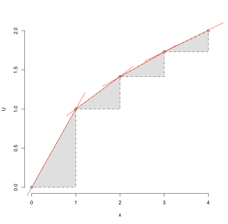
This idea is written as $M U_{x}$ , Marginal Utility. How much happiness do I gain from an increase in $x$ ? For instance, from 0 to 1 coffee, let’s say I gain 1 point of happiness. From 1 to 2 coffees, I gain 0.8 points of happiness. From 2 to 3, I gain 0.5 points of happiness, etc.

The $M U_{x}$ thus changes as our consumption increases.

We can see in the figure below, that the slope of our Utility is diminishing as we increase our consumption of $x$ . The slope is getting flatter and flatter (closer and closer to 0).

In R

x=seq(0.1, 10, by = 0.10)
x=0:10
# utility function
Ux = function(x, a) exp ( a * log(x) )
library(Deriv)
# derivative #
f_ = Deriv(Ux, "x")
df = data.frame(x, f_d = f_(x, a = 0.5), U = Ux(a = 0.5, x))
plot(df$x, df$U, xlim = c(0,4), ylim = c(0,2), xlab = 'x', ylab = "U", axes = F)
axis(side = 1)
axis(side = 2)
polygon(c(1,1,0), c(0, 1,0), col = 'gray90', lty = 4)
polygon(c(1,2,2), c(1, 1.414214,1), col = 'gray90', lty = 4)
polygon(c(2,3,3), c(1.414214, 1.732051,1.414214), col = 'gray90', lty = 4)
polygon(c(3,4,4), c(1.732051, 2.000000,1.732051), col = 'gray90', lty = 4)

The indifference curve measures the trade-off we are willing to make to keep our Utility constant; the indifference curve can also be expressed as the Marginal Utility of $x$ times the change in the consumption of $x$ (Varian, p.65-66).

Δ_{x} + M U_{x}

plus the change in the consumption of $y$ , so that our Utility does not change, $Δ U = 0$ .

M U_{x} Δ x + M U_{y} Δ y = Δ U = 0

In order word, to keep my utility constant, how much I am willing to exchange one good for another?

This rate is called the Marginal Rate of substitution (MRS). It reveals the rate at which a person is willing to substitute one good for another while maintaining the same level of utility.

\frac{Δ y}{Δ x} = - \frac{M U_{x}}{M U_{y}} = M R S

We can see from the equation above that it is the Marginal Utility (marginal enjoyment) of consuming $x$ divided by the marginal utility of consuming $y$ (see Varian p.67).

Cobbs-Douglas Utility Function

The Cobbs-Douglas Utility Function is a convex function, which means substantially that people prefer a combination of goods rather than specializing in one type of good. When specialization happens, the shape is said to be concave. With a concave shape, it “costs” more to substitute one good with another, especially at the extreme. For instance, this would apply when substituting a sport with another because one needs to learn all the rules and develop all the necessary skills to play the game.

The Cobbs-Douglas Utility Function is one of the most common functional forms.

A simple convex utility function can be defined as

U (x_{1}, x_{2}) = x_{1} \cdot x_{2}

For instance, the indifference curve can be retrieved by choosing a utility level and then solving for $x_{2}$ .

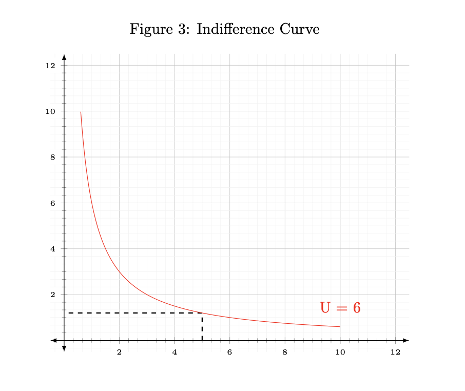
6 = 2 \cdot 3

Let’s fix the Utility to $6$ and compute all the values for $x_{2}$ .

x_{2} = \frac{U = 6}{x_{1}}

Let’s imagine $x_{1}$ goes from $1$ to $10$ units.

The keep the level of Utility at 6, we would need to have the following combinations of $x_{1}$ and $x_{2}$

\begin{array}{r} \begin{array}{rrr} x 1 & x 2 \\ 1.00 & 6.00 \\ 2.00 & 3.00 \\ 3.00 & 2.00 \\ 4.00 & 1.50 \\ 5.00 & 1.20 \\ 6.00 & 1.00 \\ 7.00 & 0.86 \\ 8.00 & 0.75 \\ 9.00 & 0.67 \\ 10.00 & 0.60 \end{array} \end{array}

All along this curve, the combinations give a fixed level of Utility of $6$ . The dotted line shows a possible combination of $x 1$ (horizontal axis) and $x 2$ (vertical axis): $(5, 1.2)$

R code

f_convex = function(x,y) x*y
# solve for y
f_convex_y = function(x,U) U/x
x = seq(0, 10, by = 1)
yU6 = f_convex_y(x, U = 6)
plot(x,yU6, type = 'l', xlim = c(0,10), ylim = c(0, 10))

Two Canonical Cobbs-Douglas expressions

Two common expressions of the Cobbs-Douglas utility function are the following

U (x_{1}, x_{2}) = x_{1}^{α} \cdot x_{2}^{b}

for example

U (x_{1}, x_{2}) = 5^{0.5} \cdot 5^{0.5} = 5

and

U (x_{1}, x_{2}) = α ln x_{1} + b ln x_{2}

U (x_{1}, x_{2}) = 0.5 ln 5 + 0.5 ln 5 = 1.609438

Which is

exp (1.609438) = 5

For the first expression, we can solve for $x_{2}$ with

x_{2} = {(\frac{U}{x_{1}^{α}})}^{\frac{1}{b}}

x_{2} = \sqrt[b]{U \cdot x^{- α}}

in R

f_cobbs = function(x,y,a,b) (x^a) * (y^b)
f_cobbs_y = function(x,U,a,b) (U / x^a)^(1/b)
f_cobbs2_y = function(x,U,a,b) (U * x^(-a))^(1/b)

And for the second expression, we can solve for $x_{2}$ with

x_{2} = exp (\frac{U - a \cdot ln x_{1}}{b})

with R

f_cobbs_ln = function(x,y,a,b) a*log(x) + b*log(y)
f_cobbs_ln_y = function(x,U,a,b) exp ( (U -  a*log(x) ) / b)

Budget

Let’s imagine that we can only pick $10$ units in total from $x_{1}$ and $x_{2}$ . The list of combinations would be

\begin{array}{r} \begin{array}{rrrr} x 1 & x 2 & x 1 + x 2 \\ 1 & 0.00 & 10.00 & 10.00 \\ 2 & 1.00 & 9.00 & 10.00 \\ 3 & 2.00 & 8.00 & 10.00 \\ 4 & 3.00 & 7.00 & 10.00 \\ 5 & 4.00 & 6.00 & 10.00 \\ 6 & 5.00 & 5.00 & 10.00 \\ 7 & 6.00 & 4.00 & 10.00 \\ 8 & 7.00 & 3.00 & 10.00 \\ 9 & 8.00 & 2.00 & 10.00 \\ 10 & 9.00 & 1.00 & 10.00 \\ 11 & 10.00 & 0.00 & 10.00 \end{array} \end{array}

If we calculate the Utility for all the combinations according to

U (x_{1}, x_{2}) = x_{1}^{α} \cdot x_{2}^{b}

We have the following Utility distribution

\begin{array}{r} \begin{array}{rrrrr} x 1 & x 2 & x 1 + x 2 & U \\ 1 & 0.00 & 10.00 & 10.00 & 0.00 \\ 2 & 1.00 & 9.00 & 10.00 & 3.00 \\ 3 & 2.00 & 8.00 & 10.00 & 4.00 \\ 4 & 3.00 & 7.00 & 10.00 & 4.58 \\ 5 & 4.00 & 6.00 & 10.00 & 4.90 \\ 6 & 5.00 & 5.00 & 10.00 & 5.00 \\ 7 & 6.00 & 4.00 & 10.00 & 4.90 \\ 8 & 7.00 & 3.00 & 10.00 & 4.58 \\ 9 & 8.00 & 2.00 & 10.00 & 4.00 \\ 10 & 9.00 & 1.00 & 10.00 & 3.00 \\ 11 & 10.00 & 0.00 & 10.00 & 0.00 \end{array} \end{array}

We can see that the maximum Utility we can reach here is $5$ “utils” from a combination of $5$ $x_{1}$ and $5$ $x_{2}$

\begin{array}{r} \begin{array}{rrrrr} x 1 & x 2 & x 1 + x 2 & U \\ 6 & 5.00 & 5.00 & 10.00 & 5.00 \end{array} \end{array}

Let’s calculate the points from an Indifference Curve with a Utility of $5$ and an Indifference Curve with a Utility of $3$ .

This would look like this

In the table below, we use the equation $x_{2} = {(\frac{U}{x_{1}^{α}})}^{\frac{1}{b}}$ to solve for $x_{2}$ , fixing $U$ at $5$ and at $3$ .

The table shows the values of $x_{2}$ (i.e. the number of units) we would need to keep our utility constant. For instance, if we look at row number 2, we have 1 unit of $x_{1}$ and $25$ units of $x_{2}$ . However, this is well above our budget.

The only combination within the budget for a Utility of $5$ , which is the maximum we can get given the Utility function $U (x 1, x 2) = x_{1}^{α} \cdot x_{2}^{b}$ , is to get $5$ units of $x 1$ and $5$ units of $x 2$ . All other combinations are over our budget.

Now if we look at the indifference curve with a Utility of $3$ ( $U = 3$ ), we see that most combinations are below our budget (except for $10$ units of $x 1$ to $0$ units of $x 2$ , or $1$ to $9$ ). This indicates that not only do we have a lower Utility on this line, $U = 3$ while we could have $U = 5$ , but we also do not make the most of our budget.

This is why the combination $5 x_{1}$ and $5 x_{2}$ is optimal. It respects our budget while maximizing our Utility.

\begin{array}{r} \begin{array}{rrrrrrr} x 1 & x 2 & x 2 with U = 5 & Budget U = 5 & x 2 with U = 3 & Budget U = 5 \\ 1 & 0.00 & 10.00 & I n f & I n f & I n f & I n f \\ 2 & 1.00 & 9.00 & 25.00 & 26.00 & 9.00 & 10.00 \\ 3 & 2.00 & 8.00 & 12.50 & 14.50 & 4.50 & 6.50 \\ 4 & 3.00 & 7.00 & 8.33 & 11.33 & 3.00 & 6.00 \\ 5 & 4.00 & 6.00 & 6.25 & 10.25 & 2.25 & 6.25 \\ 6 & 5.00 & 5.00 & 5.00 & 10.00 & 1.80 & 6.80 \\ 7 & 6.00 & 4.00 & 4.17 & 10.17 & 1.50 & 7.50 \\ 8 & 7.00 & 3.00 & 3.57 & 10.57 & 1.29 & 8.29 \\ 9 & 8.00 & 2.00 & 3.12 & 11.12 & 1.12 & 9.12 \\ 10 & 9.00 & 1.00 & 2.78 & 11.78 & 1.00 & 10.00 \\ 11 & 10.00 & 0.00 & 2.50 & 12.50 & 0.90 & 10.90 \end{array} \end{array}

Prices

Economists usually work with a price tag for goods. Let’s imagine we are dining in a restaurant, and we can get either food $x$ and food $y$ .

Our budget ( $I$ ) is $100$ dollars. A unit of food $x$ costs $3$ dollars (price $p_{x}$ ) and a unit of food $y$ costs $2$ dollars (price $p_{y}$ ).

We want to spend all of our budget tonight. The budget will be the number of units of food multiplied by their respective prices.

I = p_{x} x + p_{y} y

If I buy $20$ units of $x$ , I can only get $20$ units of $y$ (and viceversa)

y = \frac{I - p_{x} x}{p_{y}}

20 = \frac{100 - 20 \cdot 3}{2}

$ 100 = 20 \cdot $ 3 + 20 \cdot $ 2

In R

f = function(x,px,y,py) x*px + py*y
f_y = function(x,px,py, I) (I - x*px)/py

f(x = 20, px = 3, y = 20, py = 2)
# verify
f_y(x = 20, px = 3, py = 2, I = 100)

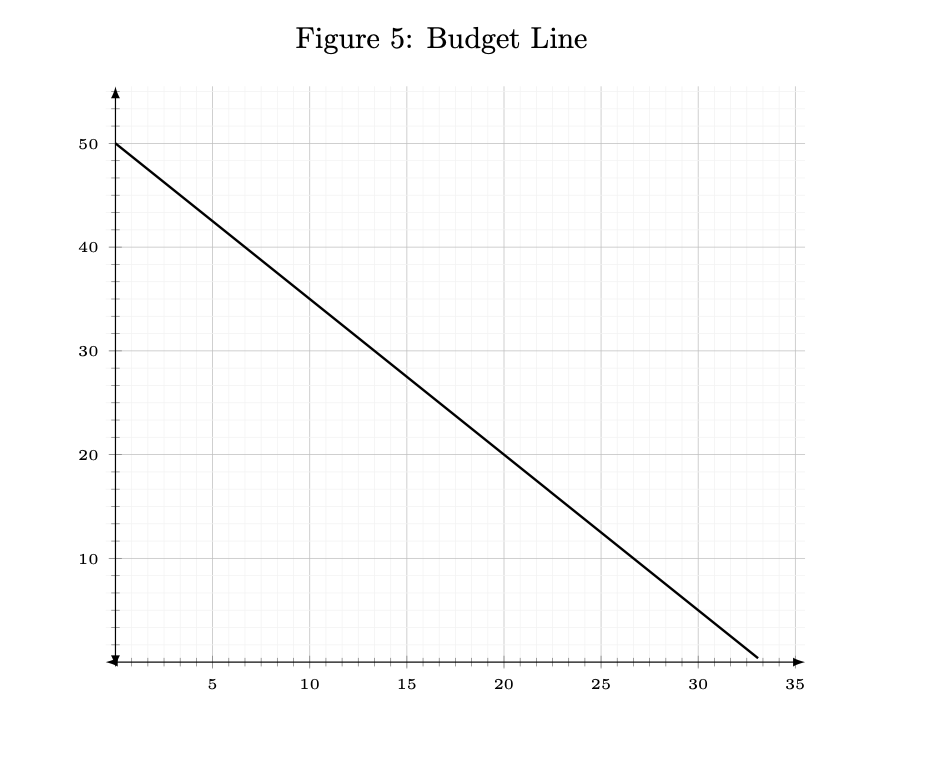
We can find the maximum units of $x$ and $y$ by calculating all our budget spent on either $x$ or $y$ .

For $x$ , we have

\frac{I}{p_{x}} = x = 33

and for $y$ ,

\frac{I}{p_{y}} = y = 50

f_max = function(I,px) I/px
f_max(I = 100, px = 3)
f_max(I = 100, px = 2)

This gives us units $33$ for $x$ ( $33.33 \cdot 3 = 100$ ) and $50$ units and for $y$ ( $50 \cdot 2 = 100$ )

We can draw our budget line with

x = 0:33
y = 50 - (px/py) * x
plot(x,y)

Imagine that, in this case, our preferences take the following form

U (x, y) = x^{0.7} \cdot y^{0.3}

Although $x$ costs more than $y$ , I derive more Utility from eating it than from eating $y$ . One way to understand the exponent is to say that for each unit of $x$ consumed, I derive $0.7$ Utility (ok, this is very abstract).

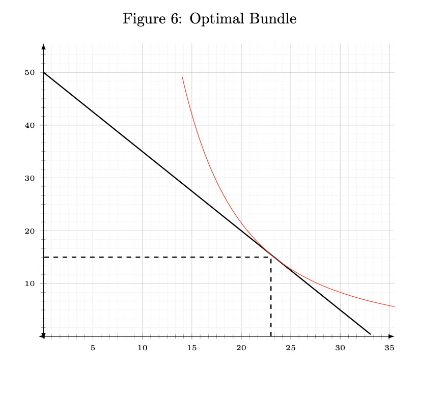
We ask: what is the optimal combination of $x$ and $y$ given our budget of $100$ dollars and our utility function?

Strategy 1

Calculate the maximum Utility from this function, draw the indifference curve of the maximum Utility and find the combination that respects the budget.

With R

x = 0:33 # max x if y is 0
y = 50 - (px/py) * x # max y if x is 0
maxU = max(f_cobbs(x = x, y = y, a = 0.7, b = 0.3))

We get $20.43$ “utils”. This is the maximum of Utility from this functional form (given $x$ and $y$ ).

Let’s predict the number of units of $y$ , given our maximum Utility

y = f_cobbs_y(x, U = maxU, a=0.7, b=0.3)
df = data.frame(x, y) %>% mutate(Budget = x*px+y*py)
w = which.min(df$Budget - 100)
df[w, ]

The combination that respects our budget is $23$ units of $x$ and $15.5$ units of $y$ .

We can verify with

f = function(x,px,y,py) x*px + py*y
f(x = 23, px = 3, y = 15.5, py = 2)

Strategy 2. Marginal Utility and Marginal Rate of Substitution

We said above that the the Marginal Rate of Substitution (MRS) is the slope of the indifference curve.

“It can be interpreted as the rate at which a consumer is just willing to substitute a small amount of good 2 for good 1.” (Varian , p.67)

MRS = Slope Budget Line

When our indifference curve’s slope equals (i.e. is tangent to) our budget line’s slope, we have the optimal combinations of $x$ and $y$ .

Varian p.75 discuss exceptions to this result.

The slope of our budget line is $- 3 / 2 = - 1.5$ .

# find maximum number of x I can get given their price
x_max = f_max(I = 100, p = px)
# find maximum number of x I can get given their price
y_max = f_max(I = 100, p = py)

Let’s create more precise values for $x$ and $y$

x = seq(0, x_max, by = 0.001)
# calculate the values for y that respect the budget #
y = y_max + (slope * x)
## plots ##
plot(x,y, type = "l", xlim = c(0,60), ylim = c(0,60))
abline(h=0,v=0, col = 'gray')
# maximum Utility
max_U = max(f_cobbs(x = x, y = y, a = a, b = b))

df2 = data.frame(x, y = f_cobbs_y(x, U = max_U, a = a, b = b)) %>% mutate(Budget = x*px+y*py)
df2$slope = slope

# indifference curve #
points(df2$x, df2$y, type = "l")

I couldn’t find how to do a partial derivative with R, so I created the following differential function

f_derive = function(h = 0.01, f = f_cobbs, x, y, a, b) (f(x = x+h, y = y, a = a, b = b) - f(x = x,y = y,a = a, b = b)) / h
MUxy = - f_derive(h = 0.01, x = x, y = y, a = a, b = b) / f_derive(h = 0.01, x = y, y = x, a = b, b = a)
df2$MRS = MUxy

w2 = which.min(abs(df2$slope - df2$MRS))
df2[w2, ]

abline(h = df2[w2, ]$y, v = df2[w2, ]$x, col = 'red')

That’s it!

Notes

Although Varian writes, “Economists have abandoned the old-fashioned view of Utility as being a measure of happiness.” (p.55), I find it helpful to still think of it in the old-fashioned way. Moreover, the field of Happiness Studies has revamped the old conception of Utility. ↩